Excel OFFSET function is an essential function for achieving dynamic ranges, and a powerful tool to create dynamic charts. These kinds of charts are able to update automatically when new data is added, so you do not have to expand the chart data source range every time you add new data.
Table of Contents
Toggle
In this tutorial, we will explore what OFFSET function is and how you can use it to create dynamic charts that adjust to changes in your data.
OFFSET Function Syntax
The OFFSET function in Excel returns a reference to a range that is offset from a starting point, by specifying the number of rows and columns to offset:
=OFFSET(reference, rows, cols, [height], [width])- reference: the starting point for the offset
- rows: the number of rows to offset from the starting position
- cols: the number of columns to offset from the starting position
- height (optional): the height of the range to return
- width (optional): the width of the range to return
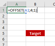
The formula above will target the cell 4 rows down and 1 column to the right in reference to cell A1.
How to Create Dynamic Charts with OFFSET
Prepare Your Data
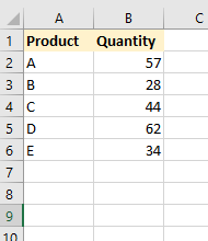
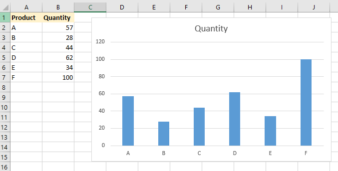
Start by organizing your data in a table format. Especially ensure that your table has column headers, so it is easy both for you and other users to interpret.
Insert a Chart
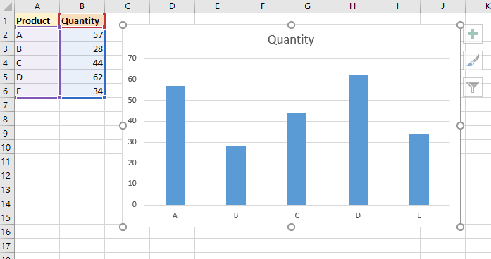
Select the data range you want to plot on the chart, including headers. Go to Insert tab on the Excel ribbon and choose the chart type.
Add Dynamic Range Names
To create a dynamic range for your chart, you can use Excel’s Name Manager option.
Go to Formulas tab on the Excel Ribbon, click on the Name Manager, and then pick New. Enter a name for your range and use the OFFSET function to create dynamic range.
You need to create 2 named ranges: 1 for X axis and the other one for chart data values.
Range 1 - Axis
To create Name Range for X axis (for products in this example table), in Name Manager we will create New Name Range called “products” and refer it to:
=OFFSET(Sheet1!$A$1;1;0;COUNTA(Sheet1!$A:$A)-1;1)This OFFSET function creates a range that will:
- Sheet1!$A$1 : start at cell A1
- 1 : skip one row (because first row is our header row)
- 0 : stay in same column
- COUNTA(Sheet1!$A:$A)-1 : have a height of a count of all the values in A column, minus 1 (header)
- 1 : have a width of 1 column
We have created our dynamic range for products. Now we need to do the similar for quantity.
Range 1 - Values
Similar to first range, create a second Name Range “quantity” and refer it to:
=OFFSET(Sheet1!$B$1;1;0;COUNTA(Sheet1!$B:$B)-1;1)Second Name Range has almost identical offset function values, just refers to column B instead of A (because our chart values are stored in column B in this example).
Connect your Chart to Ranges
With the chart selected, go to the Design tab and pick Select Data option.
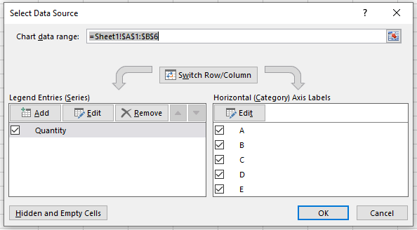
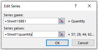
Under Legend Entries (Series) click on Edit and for Series values type name of range holding values (in our example, quantity on Sheet1).
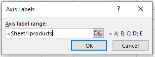
Under Horizontal (Category) Axis Labels, click on Edit and for Axis label range type name of range holding labels (in our example, products on Sheet1).
Test your chart
Now we have created a dynamic chart that will automatically update when new values are added. Let’s test it with adding new product.
Benefits of Using Dynamic Charts
- Efficiency: Dynamic charts save time by eliminating the need to manually update chart ranges when new data is added.
- Flexibility: Dynamic charts can easily accommodate changes in the size or structure of your data.
- Accuracy: By ensuring that your charts always reflect the most up-to-date data, dynamic charts help maintain data accuracy and integrity.
In conclusion, Excel’s OFFSET function offers a convenient way to create dynamic charts that automatically update to reflect changes in your data. By following the steps outlined in this tutorial, you can leverage the power of OFFSET to create more flexible and efficient data analysis tools in Excel.