Thoroughly cleaning and preparing your dataset is a crucial step in the data analysis process, as it sets it up for creating valuable insights.
Table of Contents
ToggleWe’ll go into the nuances of data cleansing using Excel in this blog post, explaining each step with real-world examples.
Before we start, it’s crucial to understand why data cleaning is indispensable step in data analysis process. Clean data forms are the essence of accurate analysis, including tasks like handling missing values, correcting errors, and maintaining uniform data formats.
Identifying and Handling Missing Data
Excel provides various tools for identifying and dealing with missing data. From simple sorting techniques to using the ‘IF’ function, you can efficiently manage missing values in your dataset. In this section, we’ll guide you through practical steps to identify and handle missing data effectively.
Imagine you’re working with a dataset tracking monthly sales, and some entries lack values. Excel equips you with various tools to pinpoint and manage missing data. Let’s say we have a sales dataset like this:
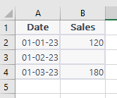
By using Excel’s ‘IF’ function, we can address missing values in the ‘Sales’ column:
=IF(ISBLANK(B2), "No Data", B2)This formula checks if a cell is blank. If it is, it displays “No Data”; otherwise, it shows the existing value.
Removing Duplicates
Duplicate entries can skew your analysis and lead to inaccurate conclusions. Excel simplifies the process of identifying and removing duplicates. We’ll walk you through the steps to ensure your dataset is free from redundant information.
Duplicate entries can be misleading. Consider a list of customer names where duplicates might exist. Excel simplifies duplicate management with its ‘Remove Duplicates’ feature. Here’s an example:
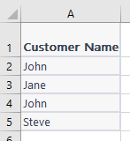
Select the column, go to the ‘Data’ tab, and click ‘Remove Duplicates.’ Excel will prompt you to select the column with duplicates, and voilà, you have a refined list.

Text-to-Columns for Data Separation
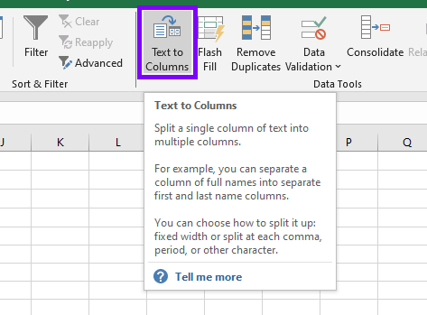
Sometimes, data in a single column needs to be split into multiple columns or combined to one column. Excel’s ‘Text-to-Columns‘ feature comes to the rescue. Learn how to use this powerful tool to separate, for instance, a combined “Name” and “Surname” column into two distinct columns.
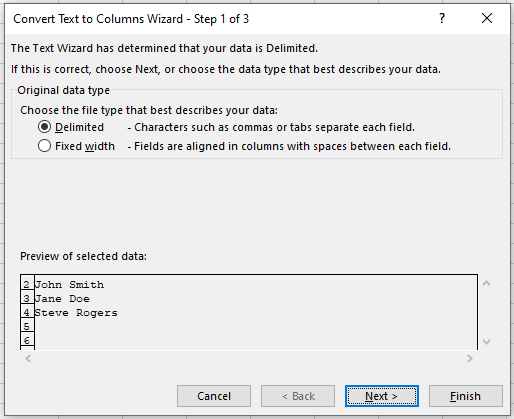
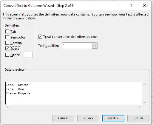
Suppose you have a dataset with combined ‘Name’ and ‘Surname’ columns. Excel’s ‘Text-to-Columns’ feature can split them swiftly:
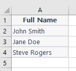
Select the column, go to ‘Data’ > ‘Text to Columns,’ choose ‘Delimited,’ select ‘Space’ as the delimiter, and Excel will create separate ‘First Name’ and ‘Last Name’ columns.
Correcting Data Errors with Find and Replace
Data entry errors are inevitable, but correcting them doesn’t have to be a headache. Excel’s ‘Find and Replace‘ function allows you to quickly rectify mistakes and ensure consistency in your dataset.
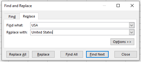
Let’s say you have a column with variations of “United States” like “USA” or “U.S.A.” Utilize ‘Find and Replace’ to standardize:
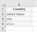
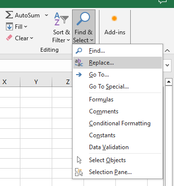
Go to Home tab, and under Find & Select, pick Replace option (or use Ctrl + H keyboard shortcut). Enter “USA” in ‘Find What,’ and “United States” in ‘Replace With.’ Excel will swiftly replace all instances.
Utilizing Excel Formulas for Data Transformation
Excel’s array of formulas can be harnessed for data transformation. From ‘CONCATENATE’ to ‘IFERROR,’ we’ll explore how these formulas can help you derive new insights or clean up your dataset effortlessly.
Consider a scenario where you have separate ‘First Name’ and ‘Last Name’ columns, and you wish to create a unified ‘Full Name’ column. Excel’s CONCATENATE function comes to your rescue:
=CONCATENATE(A2, " ", B2)In this formula, assuming ‘First Name’ is in column A and ‘Last Name’ is in column B, CONCATENATE joins the two with a space in between. The result in the ‘Full Name’ column would be “John Smith.”
The IFERROR function is a handy tool for dealing with potential errors in formulas. Let’s say you’re calculating the ratio of ‘Revenue’ to ‘Expenses,’ but some ‘Expenses’ values are zero, risking a division by zero error. The IFERROR function can prevent this issue:
=IFERROR(A2/B2, "N/A")In this formula, if there’s an error in the division (for example, if ‘Expenses’ (B2) is zero), it displays “N/A” instead of an error message. This enhances the robustness of your data analysis by gracefully handling potential pitfalls.
Creating PivotTables for Summary Analysis
Once your data is clean, organizing it for analysis becomes more straightforward. PivotTables in Excel offer a dynamic way to summarize and analyze data.
Suppose you have a dataset of daily sales:
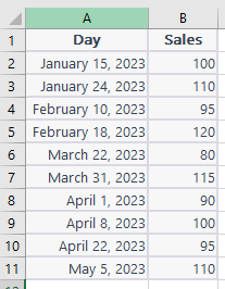
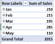
Select the data, go to ‘Insert’ > ‘PivotTable,’ and you can analyze total sales per month effortlessly.
Data analysis is only as good as the data you start with. By mastering cleaning and preparing your data in Excel, you lay the groundwork for accurate, insightful analyses. Knowing these Excel techniques, you’re well on your way to extracting valuable insights from your data.


