Adding Trendlines and Data Labels to Charts

Trendlines and data markers can provide valuable insights and enhance the visual representation of your data in Excel charts. Trendlines help you identify patterns and trends in your data, while data markers provide individual data points for better clarity.

Table of Contents

Add Trendlines

1. Select the chart that you want to change. Within “Chart Tools” bar, “Chart Design”, find the “Add Chart Element” button. Click on it to reveal a dropdown menu.

2. From the dropdown menu, select “Trendline” and choose the desired trendline type, such as linear, exponential, logarithmic, or moving average.

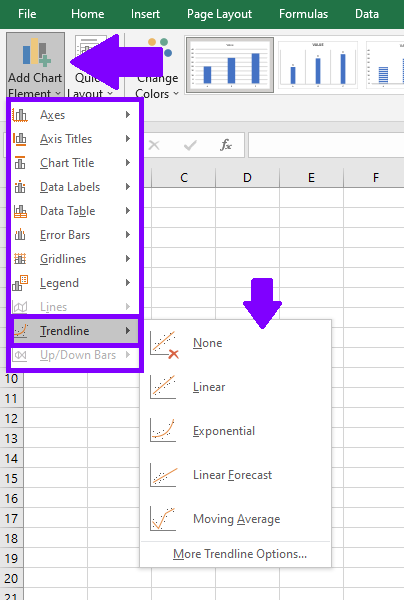
3.Excel will add the trendline to the chart, displaying the best-fit line or curve based on your selected trendline type.

You can customize the trendline by right-clicking on it and selecting "Format Trendline" to adjust settings such as line style, color, and more.

Add Data Labels

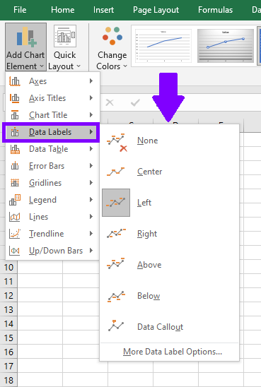
1. To add data labels to your chart, find the “Data Labels” button in the “Add Chart Element” group.

2. Click on the “Data Labels” button and choose the desired data label option.

3. Excel will add data markers to your chart, showing individual data points for better visibility.

You can further customize the data markers by right-clicking on them and selecting "Format Data Labels" to adjust settings like position, font style, number format, and more.

By adding trendlines, you can identify trends, forecast future values, and analyze the relationship between variables in your data. Data labels, on the other hand, help you visualize individual data points and provide additional context. Experiment with different trendline types and data labels options to effectively communicate your data insights and create best user report experience.