Conditional Formatting - datalitico.com

Excel is a powerful tool for organizing and analyzing data. However, it can be difficult to spot important data within large sets of information. That’s where conditional formatting comes in.

Table of Contents

Conditional formatting is a feature in Excel that allows you to automatically highlight cells based on specific criteria. This can help you quickly identify important data and draw attention to key insights.

How to apply Conditional Formatting

Select the range of cells to which you want to apply conditional formatting.
Go to the “Home” tab in the Excel ribbon. In the “Styles” group, click on the “Conditional Formatting” button. A drop-down menu will appear with various conditional formatting options.
Choose the desired conditional formatting rule from the menu. Excel provides several pre-defined rules, such as highlighting cells that contain specific text or values, highlighting top or bottom values, data bars, color scales, and more. You can select one of these rules, or click on “New Rule” to create a custom rule.
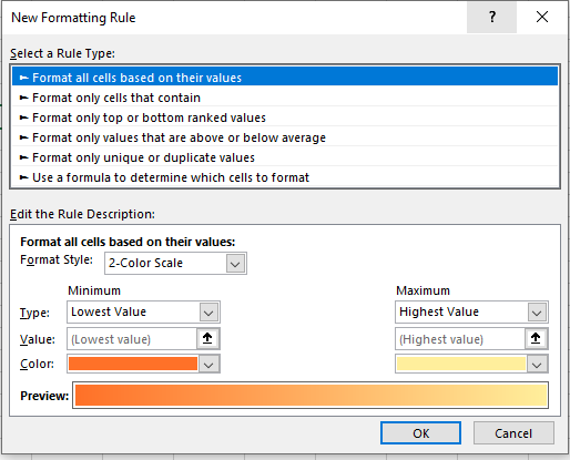
Configure the settings for the selected rule.
Customize the formatting options. Depending on the rule, you can choose the font color, cell color, border style, data bar color, or icon set to apply to the cells that meet the specified condition.
Preview the changes in the “Preview” section of the dialog box to see how they will affect your selected cells.
Once you have configured the conditional formatting rule and formatting options, click the “OK” button to apply the conditional formatting to the selected cells.

Let’s highlight all numbers greater than 10 in red.

Creating Custom Formatting Rules

If the pre-set formatting rules don’t meet your needs, you can create your own custom rule. To do this, select “New Rule” from the Conditional Formatting menu. There are many available options to create custom formatting rule.

To create a rule that highlights cells containing a specific word or phrase, such as "urgent" in cell range D4:D8. To do this, select "New Rule" from the Conditional Formatting menu, and choose "Use a formula to determine which cells to format."

Then, enter a formula that specifies the criteria for highlighting cells. For example, to highlight cells containing the word "urgent," you could enter the formula =SEARCH("urgent";D4:D8)>0.

Data Bars and Color Scales

In addition to applying specific formatting to cells, you can also use data bars and color scales to visually represent your data. Data bars are graphical representations of values in a cell that can be used to quickly see how different values compare to one another. Color scales are similar, but use colors instead of bars to represent data.

You can use a green-to-red color scale to represent values that range from low to high.

To apply data bars or color scales, select the cells you wish to format and choose "Data Bars" or "Color Scales" from the Conditional Formatting menu. You can then choose a pre-set style or create your own custom style. Once you have applied your formatting, you can easily see how different values compare to one another and identify trends in your data.

You can add multiple conditional formatting rules to the same range of cells. The rules will be evaluated in the order they were applied, so make sure to arrange them accordingly if you have specific priorities.

Conditional formatting provides a powerful way to visually analyze and highlight important aspects of your data. By using this feature, you can quickly identify trends, outliers, or specific patterns that may be critical for your analysis.