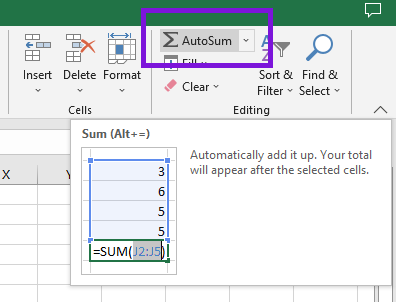
The AutoSum feature in Excel is a convenient tool that allows you to quickly calculate the sum of a range of cells without manually typing the SUM formula. It automatically suggests the most likely range of cells to sum based on the data in your worksheet. Using the AutoSum feature can save you time and effort when performing basic calculations. Here’s how to use it.
1. Select the cell where you want the sum to appear. For example, if you want the sum to appear in cell B1, click on that cell to select it.
2. Look for the “AutoSum” button in the “Editing” group on the Excel ribbon. It is usually located on the Home or Formulas tab, depending on your Excel version. The button is represented by the Greek letter sigma (∑) next to an arrow pointing downwards.

3. Click on the AutoSum button. Excel will automatically select what it believes is the range of cells you want to sum based on the adjacent data. The selected range will have a marquee border around it.
4. Press Enter on your keyboard to confirm the AutoSum selection. Excel will insert the SUM formula in the selected cell, adding up the values within the range it identified.
5. If the AutoSum selection is not correct, you can manually adjust the range. Simply click and drag the mouse to select the desired range of cells you want to sum. The selected range will update in the formula bar at the top of the Excel window.
6. Press Enter on your keyboard to confirm the adjusted range and calculate the sum using the modified selection.
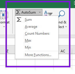
The AutoSum feature can also be used to calculate other types of calculations, such as averages, counts, and more. After clicking the AutoSum button, you can choose from a drop-down menu of other functions available for quick selection.

By utilizing the AutoSum feature, you can save time and reduce the chances of errors when performing basic calculations in Excel. It is a handy tool for quickly getting the sum or other calculations without the need to manually write formulas.

